Environmental Engineering Reference
In-Depth Information
20
18
16
14
12
10
8
6
4
2
0
0
5
10
15
20
F
-1
[F
n
(
d
2
m
)]
χ
2
m
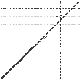
Figure 1.29
Line test for the transformed (
X
1
,
X
2
,
X
3
) data.
1.6.5 Simulation
Given the identified types and parameters in
Table 1.15
and the estimated correlation matrix
lowing steps:
1. Simulate independent standard normal random vector
Z
= [Z
1
, Z
2
, Z
3
]
T
.
2. Let
u
matrix be the Cholesky decomposition of
C:
(1.106)
uu
T
×=
C
In MATLAB,
u
= chol(
C
).
3. Let
(1.107)
XZu
T
=×
1.6.6 Some practical observations
Can we simulate (Y
1
, Y
2
, Y
3
) without considering the correlations among (Y
1
, Y
2
, Y
3
)? This
can be done by simulating each Yi
i
separately. However, it is wrong to ignore such correla-
tions, namely, set δ
12
= δ
13
= δ
23
= 0 in violation of nonzero correlations exhibited by the
tions.
Figure 1.30
should be compared to
Figure 1.25
. It is clear that the correlations shown
in
Figure 1.25
are not observed in
Figure 1.30
.
shows the simulated (Y
1
, Y
2
, Y
3
) data. It is clear that deterministic correlations exist among
(actual data). Note that δ
12
, δ
13
, and δ
23
are the Pearson product-moment correlations among
(X
1
, X
2
, X
3
). They are not the Pearson correlations among (Y
1
, Y
2
, Y
3
). The Pearson correla-
tions among the (Y
1
, Y
2
, Y
3
) data shown in
Figure 1.31
are, surprisingly, not 1. In fact, they
Search WWH ::

Custom Search