Environmental Engineering Reference
In-Depth Information
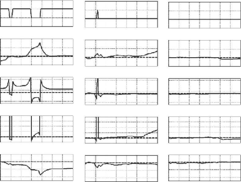
1.5.5 Some practical observations
1.5.5.1 Choice of z
Previously, we have chosen
z
= 0.7, which is recommended in Slifker and Shapiro (1980). It
turns out that this choice is robust.
Figure 1.23
shows the variation (with respect to
z
) of
the identified distribution type and (
a
X
,
b
X
,
a
Y
,
b
Y
) for
one realization
of the simulated Y
data. For plotting on a numerical scale, SU is indexed as “1,” SB is indexed as “2,” and SL
is indexed as “3.” The values for the actual Y distribution (namely, type = 1,
a
X
= 1,
b
X
= −1,
a
Y
= 1, and
b
Y
= 0) are plotted as dashed lines. The effect of sample size is illustrated in the
subplots using
n
= 30, 100, and 1000. When
n
= 30, the identified type is incorrect regard-
less of the choice of
z
. This false identification is less severe when
n
= 100. However, we
still see few false identifications when
z
is near 0.4. There is no false identification when
n
= 1000. The identified (
a
X
,
b
X
,
a
Y
,
b
Y
) for
n
= 30 are very different from the actual values
because the type has been identified wrongly. The effect of these parameters on the PDF is
dependent on the probability model (
Figure 1.20
)
. The identified (
a
X
,
b
X
,
a
Y
,
b
Y
) for
n
= 100
are close to the actual values for
z
= 0.5-0.8. The identified (
a
X
,
b
X
,
a
Y
,
b
Y
) for
n
= 1000
are close to the actual values for a broad range of
z
. In general,
z
= 0.7 seems to be a robust
choice for
n
= 100 and 1000. Note that the subplot for
n
= 30 and possibly
n
= 100 will
change from realization to realization due to statistical uncertainty.
(a)
(b)
(c)
3
3
3
2
2
2
1
1
1
0
0.3
0.3
0
0.3
0.4
0.5
0.6
0.7
0.8
0.9
1
0.4
0.5
0.6
0.7
0.8
0.9
1
0.4
0.5
0.6
0.7
0.8
0.9
1
z
z
z
3
3
3
2
2
2
1
1
1
0
0.3
0
0.3
0.3
0.4
0.5
0.6
0.7
0.8
0.9
1
0.4
0.5
0.6
0.7
0.8
0.9
1
0.4
0.5
0.6
0.7
0.8
0.9
1
z
z
z
5
5
5
0
0
0
-5
-5
-5
0.3
0.4
0.5
0.6
0.7
0.8
0.9
1
0.3
0.4
0.5
0.6
0.7
0.8
0.9
1
0.3
0.4
0.5
0.6
0.7
0.8
0.9
1
z
z
z
5
4
3
2
5
4
3
2
1
0
5
4
3
2
1
0
1
0
0.3
0.4
0.5
0.6
0.7
0.8
0.9
1
0.3
0.4
0.5
0.6
0.7
0.8
0.9
1
0.3
0.4
0.5
0.6
0.7
0.8
0.9
1
z
z
z
2
0
-2
-4
2
0
-2
-4
2
0
-2
-4
0.3
0.4
0.5
0.6
0.7
0.8
0.9
1
0.3
0.4
0.5
0.6
0.7
0.8
0.9
1
0.3
0.4
0.5
0.6
0.7
0.8
0.9
1
z
z
z
n
= 30
n
= 100
n
= 1000
Figure 1.23
Variations of the identified type and (
a
X
,
b
X
,
a
Y
,
b
Y
) for
one realization
of the simulated Y data
with (a)
n
=
30; (b)
n
=
100; and (c)
n
=
1000.
Search WWH ::

Custom Search