Environmental Engineering Reference
In-Depth Information
and practical constraints imposed by the multivariate model, which is the
final goal
in the
characterization of geotechnical engineering data.
1.5.2 non-normal distribution
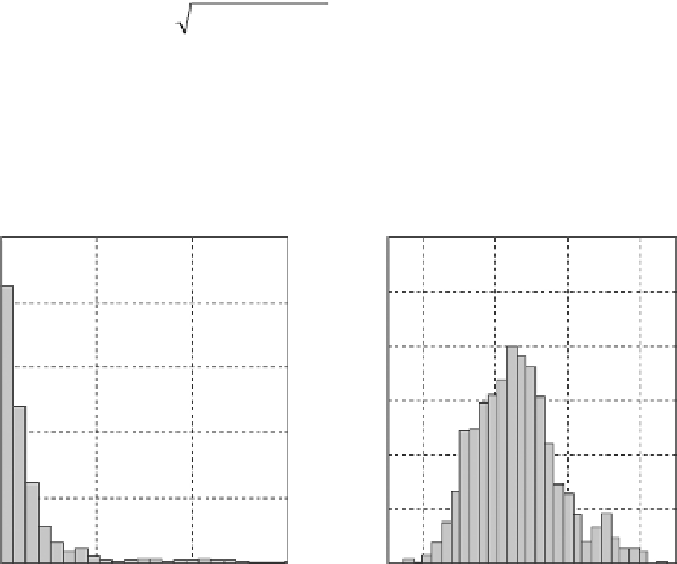
It is quite unlikely for real data points to follow the normal distribution. As explained above,
this is partly because most soil parameters are non-negative (e.g., soil shear strengths, effec-
tive stresses, moduli, etc.). Consider the normalized preconsolidation stress ( ′
/P ;
P
a
is one
atmosphere pressure) data points in the Clay/10/7490 database (Ching and Phoon 2014a).
This database contains 2028 data points for the normalized preconsolidation stress. Its his-
togram is shown in the left plot in
Figure 1.19
.
The histogram obviously does not resemble
a normal distribution. In fact, even when the natural logarithm is applied, the histogram
of ln
(
σ
pa
/P
still exhibits a certain degree of asymmetry, which is not consistent with the
normal model. In this example, there are sufficient data points for one to suspect that these
departures from normality are not caused by statistical uncertainties. We cover the Johnson
system of distributions below, starting with the lognormal distribution, which is the most
well-known member in the geotechnical engineering literature.
σ
pa
′
)
1.5.2.1 Lognormal and shifted lognormal distributions
Let Y be a nonnegative soil parameter. It is clear that Y cannot be normal. The simplest dis-
tribution model for Y is the lognormal distribution. If Y is lognormal, ln(Y) is normal with
mean = λ and standard deviation = ξ:
µ
2
λ=
ln
ξ
=
ln(
1
+
COV
)
(1.81)
1
+
COV
2
where μ and COV are the mean value and COV of Y. As a result, the relationship between
the standard normal X and Y is as follows:
1000
300
n
= 2028
n
= 2028
250
800
200
600
150
400
100
200
50
0
0
0
10
20
30
-2
0
2
4
σ′
p
/
P
a
ln(σ′
p
/
P
a
)
Figure 1.19
Histograms for
/
P
and ln(
σ
pa
′
σ
p
′
/
).


Search WWH ::

Custom Search