Environmental Engineering Reference
In-Depth Information
Table 1.13
Mean, COV, and standard deviation for
s
u
,
′
σ
p
N, and
q
t
−
σ
v
Variable
μ
COV
σ
Undrained shear strength
s
u
200 kPa
0.2
40 kPa
Preconsolidation stress
800 kPa
0.2
160 kPa
σ
p
′
SPT blowcount
SPT-N value
20
0.3
6
Net cone tip resistance
2500 kPa
0.3
750 kPa
q
t
−
σ
v
where μ's and σ's are the mean values and standard deviations, respectively, listed in
Table
chosen such that
s
up
σ
p
P
/ /N0
(P
a
= 101.3 kPa is
the atmosphere pressure). These values are typical (e.g., Kulhawy and Mayne 1990). Let us
further assume the correlation matrix
C
for (X
1
, X
2
, X
3
, X
4
) is
/
σ
′ ≈
0.
25
,(
q
−
σ
)
/
s
≈
25
. ,
and
(
′
)
≈
.
t
v
u
1090507
09 10406
05 04 104
07 06 04
.
.
.
.
.
.
C
=
(1.73)
.
.
.
.
.
.
1
Suppose site investigation yields the following information at a certain depth in a clay
layer: N = 10 and
q
t
- σ
v
= 2000 kPa. On the basis of this information, the purpose is to
update the marginal distributions of
s
u
and
σ
p
for the clay at the same depth. The uncon-
ditional distribution for
s
u
is normal with mean = 200 kPa and COV = 0.2. The updated
(conditional) distribution for
s
u
is expected to be different.
The effect of updating (or conditioning) can be explained by simulated data. A large
amount (
n
= 2 × 10
6
) of (, ,,
′
N − data are simulated. This can be done by first
simulating
Z
= normrnd(0, 1,
n
, 4). Then, the Cholesky factor is computed as
u
= chol(
C
).
Finally,
X
T
=
Z
T
×
u
. The first column in
X
contains the X
1
samples; so,
s
u
= μ
1
+ σ
1
× X
1
will yield
n
= 2 × 10
6
samples of
s
u
. The same procedure will yield
n
= 2 × 10
6
samples of ′
s
σ
′
q
σ
)
up
t
v
σ
p
N, and
q
t
- σ
v
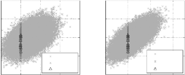
. These samples are plotted as light-gray crosses in
Figure 1.16
.
It is clear that
(
s
u
, N) are positively correlated, and so are (
s
u
,
q
t
- σ
v
). These are the unconditional samples
400
400
300
300
200
200
No info
100
100
No info
q
t
-
σ
v
info
SPT-N info
Both info
Both info
0
0
0
0
10
20
N
30
40
2000
4000
6000
q
t
-
σ
v
(kPa)
Figure 1.16
Illustration of conditioning using simulated (
s
u
, N,
q
t
−
σ
v
) samples.


Search WWH ::

Custom Search