Application of the subset simulation approach to spatially varying soils - Risk and Reliability in Geotechnical Engineering - page 560

(a) 9 (b) 240

210
180

8
7
6
5
4

150
120
90
60
30
0

3
2
1
0

0 500 1000 1500 2000 2500 3000 0 500 1000 1500 2000 2500 3000

N s N s

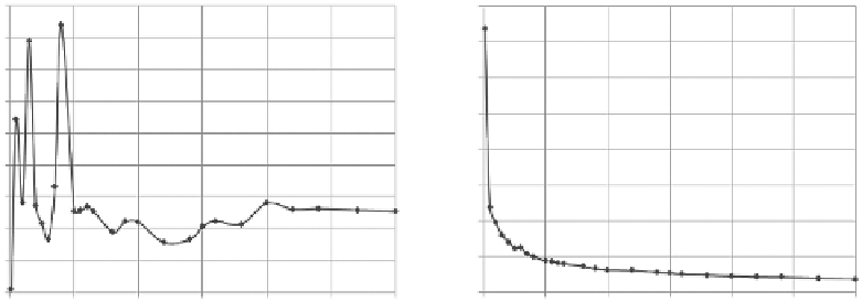
Figure 15.3 Pf f and COV( P f ) versus the number of realizations N s .

Figure 15.3b shows the effect of N s on the coefficient of variation of the failure probability
COV Pf . As expected, COV Pf decreases with increasing N s . Notice that the values of COV Pf
for N s = 2200 and 2400 samples are equal to 12.8 and 12.4%, respectively, which indicates
(as expected) that the COV Pf decreases with the increase in the number of realizations.
It should be mentioned here that for p 0 = 0.2, four levels of SS were found necessary
to reach the limit state surface G = 0 as may be seen from Table 15.6 . Therefore, when
N s = 2200 samples, a total number of N t = 2200 × 4 = 8800 samples were required to calcu-
late the final P f value. Remember that in this case, the COV of P f was equal to 12.8%. Notice
that if the same value of COV (i.e., 12.8%) is desired by MCS to calculate P f , the number of
samples would be equal to 20,000. This means that, for the same accuracy, the SS approach
reduces the number of realizations by 56%. On the other hand, if one uses MCS with the
same number of samples (i.e., 8800 realizations), the value of COV of P f would be equal
to 19.6%. This means that for the same computational effort, the SS approach provides a
smaller value of COV( P f ) than MCS.

15.5.3 example 3: Computation of the failure probability
by an SS approach in the case of random fields
This section presents a probabilistic analysis at the serviceability limit state (SLS) of a strip
footing resting on a spatially varying soil using the SS approach. The objective is the compu-
tation of the probability P e of exceeding a tolerable vertical displacement under a prescribed
footing load. Only one soil variability ( l ln x = 10 m and l ln y = 1 m) is considered in this sec-
tion. An extensive probabilistic parametric study on the same problem may be found in
Ahmed and Soubra (2012).
A footing of breadth b = 2 m that is subjected to a central vertical load P s = 1000 kN/m
(i.e., an applied uniform vertical pressure q s = 500 kN/m 2 ) was considered in the analysis.
As in Example 1, the Young's modulus was modeled by a random field and it was assumed
to follow a log-normal PDF. The mean value and the coefficient of variation of the Young's
modulus were, respectively, μ E = 60 MPa and COV E = 15%. An exponential covariance
function was used to represent the correlation structure of the random field. The random
field was discretized using K-L expansion. The performance function used to calculate the
probability P e of exceeding a tolerable vertical displacement was defined as follows:

G = δ v max − δ v (15.21)