Constructing multivariate distributions for soil parameters - Risk and Reliability in Geotechnical Engineering - page 24

(a) 4 (b) 4

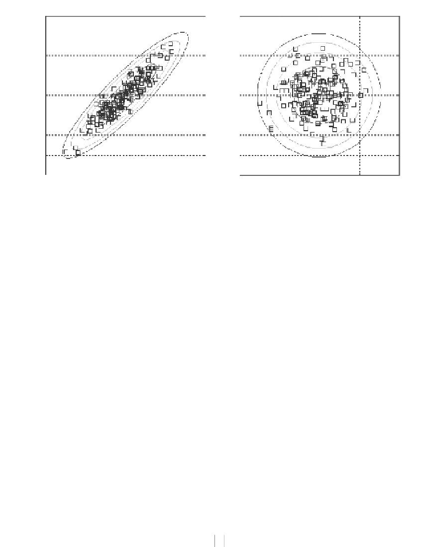
δ 12 = 0.9
n = 200

δ 12 = 0
n = 200

3 3

2 2

1 1

0 0

-1 -1

-2 -2

-3 -3

- -4 - -4

-2 0 2 4 -2 0 2 4

X 1 X 1

δ 12 = 0.9 δ 12 = 0

Figure 1.12 Contour plots for the bivariate standard normal distribution of (X 1 , X 2 ).

( ) ⋅ ( )

∑

n

() k () k

1 ( n − 1 ) X − m X − m

1 1 2 2

k = 1

δ 12 ≈

(1.40)

( ) ( )

∑

n 2

∑

n 2

() k () k

1 ( n − 1 ) X − m × 1 ( n − 1 ) X − m

1 1 2 2

k = 1 k = 1

where the superscript ( k ) is the sample index; m i is the sample mean of Xi. i . Note that the
denominator is simply the product of the sample standard deviation of X 1 and the sample
standard deviation of X 2 . The MATLAB function corr( X 1 , X 2 ,'type', 'Pearson') and the
EXCEL command CORREL( X 1 , X 2 ) can be used to find the δ 12 estimate in Equation 1.40 .
Here, X 1 = …

( )

T

X X

() 1

, ,

() n

is an ( n × 1) vector that contains all samples of X 1 .

1 1

1.3.3.2 Maximum likelihood method
The maximum likelihood method can also be employed:

n

1

∏

( ) ( )

T

µσδ , , ≈ argmax exp. −× − 05 X k

()

µ CX

− 1 () k

− µ

MLE LE 12 , MLE

2

2 π ⋅ C

µµσσδ , , , ,

1 21212

k = 1

n

∑

( ) −

( )

T

( )

= argmax − ln CX

( k )

− µ CX

− 1 ( ) k

− µ (1.41)

µµσσδ , , , ,

1 21212

k = 1

where

() k

=

X
X

=

µ
µ

=

σ

2

δσσ

1

1 1 12 12

X

() k

µ C

(1.42)

() k

δσσ σ

2

2

2 12 12 2