Environmental Engineering Reference
In-Depth Information
(a)
20
(b)
20
(c)
30
25
15
15
20
15
10
10
10
5
5
5
0
0
0
0
0
0
100
y
200
100
y
200
100
y
200
n
=
30
n
=
50
n
=
100
Figure 1.5
Histograms of Y with three different sample sizes (
n
).
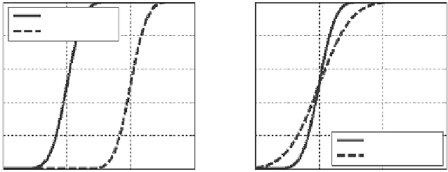
The concept of a CDF and its associated S-shaped curve should be familiar to all geo-
technical engineers. It is identical to the grain size distribution, which plots the percent-
age finer by weight versus grain diameter. F(
y
) can be evaluated using EXCEL function
NORMDIST(
y
, μ, σ, 1) or MATLAB function normcdf(
y
, μ, σ). When μ increases from 100
(stiff clay) to 200 kPa (very stiff clay), the curve shifts to the right (
Figure 1.6a
). When σ
increases from 20 (low variability with COV = 20%) to 40 kPa (medium variability with
COV = 40%), the curve becomes less steep (
Figure 1.6b
).
For standard normal X, the CDF is denoted by Φ(
x
):
x
1
2
−
t
2
⋅
∫
Φ()
x
=
exp
dt
(1.6)
2
π
−∞
Φ(
x
) can be evaluated using EXCEL function NORMSDIST(
x
, 1) or MATLAB function
normcdf(
x
). It is noteworthy that F(
y
) can be computed from Φ by appropriate shifting and
scaling
y
−
µ
y
−
µ
F
()
y
=
P Y
(
≤ =+≤= ≤
y
)
P
(
µσ
X
y
)
P X
=
Φ
(1.7)
σ
σ
(a)
1
(b)
1
μ
= 100,
σ
= 20
μ
= 200,
σ
= 20
0.8
0.8
0.6
0.6
0.4
0.4
0.2
0.2
μ
= 100,
σ
= 20
μ
= 200,
σ
= 20
0
0
0
0
100
200
300
100
200
300
y
y
Effect of µ
Effect of µ
Figure 1.6
CDFs of normal random variables.


Search WWH ::

Custom Search