Environmental Engineering Reference
In-Depth Information
0.55
(1) Load bias statistics
μ
XQ
= 1.00
COV
XQ
= 0.283
(1)
(2)
0.50
β
= 2.33 (P
f
= 0.01)
(2) Load bias statistics
μ
XQ
= 1.20
COV
XQ
= 0.108
0.45
0.40
0.384
β
= 3.09 (P
f
= 0.001)
(1)
(2)
0.35
0.30
Resistance bias statistics
μ
XR
= 1.00
COV
XR
= 0.356
0.25
0.20
1.0
1.1
1.2
1.3
1.4
1.5
Load factor,
γ
Q
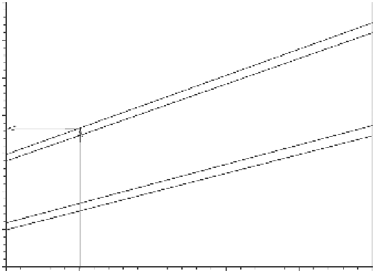
Figure 8.8
Example outcomes for resistance factor
φ
using closed-form solution.
argued to be small, but recall that the load and resistance models used here were judged to
be good models because they were originally calibrated to: (a) give mean bias values close
to 1; (b) minimize the spread in bias values; and (c) remove bias dependencies with pre-
dicted values. Poorer models with greater differences between fit-to-tail and fit-to-all data
can be expected to give larger differences in calculated resistance factor. Furthermore,
many load and resistance models used in ASD past practice are poor candidates for LRFD
calibration because the mean load bias values are so low that in order to satisfy a reason-
able target β value during calibration, the resistance factor value must be greater than 1.
This is contrary to expectations of design engineers using current LRFD design codes in
North America.
The inverse of the slopes of the lines plotted in
Figure 8.8
are equivalent to the fac-
tor of safety F = γ
Q
/φ in ASD past practice. For β = 2.33, F = 2.87-2.94 and for β = 3.09,
F = 3.87-4.02. For steel strip walls, AASHTO (2012) recommends γ
Q
= 1.35 and φ = 0.90.
These values were selected to give F = 1.5 in order to be consistent with ASD past practice.
This value is very much lower than the values computed using F = γ
Q
/φ. The difficulty of
relating LRFD calibration outcomes that are based on reliability-based theory to factor of
safety values used in ASD past practice is typical. Nevertheless, in this particular example,
it can be argued that the new load and pullout models will result in safer structures based
on the conventional notion of factor of safety in ASD past practice.
This chapter has demonstrated that judgment plays an important role in the selection of
data used to perform LRFD calibration. One example is the treatment of possible outliers.
Outliers located at the lower tail of a resistance bias CDF plot and the upper tail of a load
bias CDF plot should receive special attention because it is the distribution of bias values at
these locations that largely influence calibration outcomes. Removing bias values at these
tails when they have been taken from different case studies with no documented evidence
for rejection could lead to non-conservative LRFD calibration outcomes. Proper documen-
tation of measurement data cannot be over-stated in order that proper assessment of the
validity of all data points in measured load and resistance sample populations can be made
(Allen et al. 2005).
Search WWH ::

Custom Search