Practical reliability analysis and design by Monte Carlo Simulation in spreadsheet - Risk and Reliability in Geotechnical Engineering - page 325

450

18%

Failure sample frequency
Nominal distribution %

400 16%

14%

350

12%

300

250 10%

8%

200

150 6%

100 4%

2%

50

0 0%

S uL bin

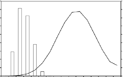
Figure 7.15 Histogram of the S uL failure samples from Subset Simulation.

(i.e., P ( F | S uL ) in Figure 7.14) obtained from Bayesian analysis is a variation of failure prob-
ability as a function of S uL . Figure 7.14 shows that, as S uL increases from 13 to 21 kPa,
the slope failure probability decreases from more than 10% to about 0.1%. It is obvious
that the values of S uL have significant effects on slope failure probability. Such effects are
explicitly quantified from the Bayesian analysis of failure samples. Variations of failure
probability as a function of S uL shown in Figure 7.14 can also be obtained from repeated
simulation runs with different deterministic S uL value in each run. Figure 7.14 also includes
results from such repeated simulation runs by open triangles. The open triangles follow
a trend similar to the open squares (i.e., the Bayesian analysis results). This validates the
Bayesian analysis results.
Figure 7.15 shows an S uL histogram of the 1134 failure samples from Subset Simulation
and a nominal (unconditional) probability distribution of S uL (i.e., a normal probability

250 18%

Failure sample frequency
Nominal distribution %

16%

200

14%

12%

150

10%

8%

100

6%

4%

50

2%

0 0%

T cr bin

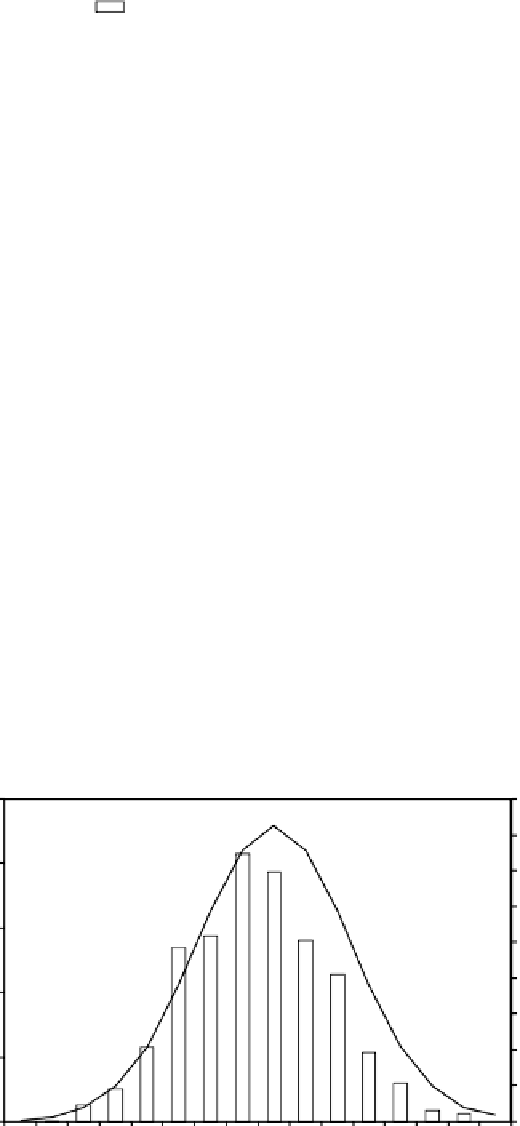
Figure 7.16 Histogram of the T cr failure samples from Subset Simulation.