Environmental Engineering Reference
In-Depth Information
α
α
α
(a)
1
0.75
0.5
Increasing p
Increasing p
Increasing p
X
1
X
1
X
1
(b)
≤ 3
≤ 4
≤ 5
≤ 6
α
α
α
α
1
1
1
1
6
6
6
6
0
0
0
0
0
6
0
6
0
6
0
6
α
≤ 3
α
≤ 4
α
≤ 5
α
≤ 6
0.75
0.75
0.75
0.75
6
6
6
6
0
0
0
0
0
6
0
6
0
6
0
6
α
≤ 3
α
≤ 3
α
≤ 3
α
0.5
≤ 3
0.5
0.5
0.5
6
6
6
6
0
0
0
0
0
6
0
6
0
6
0
6
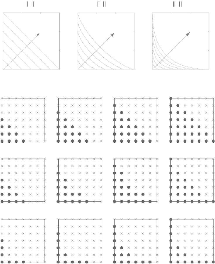
Figure 6.3
Hyperbolic truncation scheme. (After Blatman, G. and B. Sudret. 2011a.
J. Comput. Phys. 230,
2345-2367.)
The principle of LAR is to (i) select a
candidate set
of polynomials A, for example, a given
hyperbolic truncation set as in
Equation 6.48
, and (ii) build up from scratch a sequence of
sparse bases having 1, 2, …, card A terms. The algorithm is initialized by looking for the
basis term that is the most correlated with the response vector
Y
. The correlation is practi-
cally computed from the realizations of
Y
(i.e., the set Y of QoI in
Equation 6.30
)
and the
by normalizing each column vector into a zero-mean, unit variance vector, such that the
correlation is then obtained by a mere scalar product of the normalized vector. Once the
first basis term Ψ
α
1
is identified, the associated coefficient is computed such that the residual
Yy
()
Ψ
X
becomes equicorrelated with two basis terms (
This will define the
−
()
ΨΨ
α
).
α
α
α
1
2
1
1


Search WWH ::

Custom Search