Environmental Engineering Reference
In-Depth Information
5.4.3 bayesian updating with structural reliability methods
The BUS method proposed in Straub and Papaioannou (2014) is based on ideas already
presented in Section 5.3.5. The likelihood function
L(
x
) can be represented in the form of
an LSF
h
(
x
,
p
) =
p
−
cL
(
x
) in the augmented outcome space of
X
and
P
, where
P
is a stan-
dard uniform random variable and c is a constant that ensures
cL
(
x
) ≤ 1 for any
x
. It can
be shown that the posterior distribution of
X
corresponds to the prior distribution of
X
censored in the domain {
h
(
x
,
p
) ≤ 0}. The BUS approach uses structural reliability methods
to efficiently evaluate the posterior distribution defined in this way.
In its simplest form, the BUS approach reduces to the classical rejection-sampling algo-
rithm where the prior distribution is applied as an envelope distribution and the likelihood
is applied as a filter (Smith and Gelfand 1992). It can be summarized as follows (where
K
=
total number of samples from the posterior).
Simple rejection-sampling algorithm
1.
k
= 1.
f
X
().
2. Generate a sample
x
(
k
)
from
′
3. Generate a sample
p
(
k
)
from the standard uniform distribution in [0,1].
4. If
h
(
x
()
k
,
p
()
k
)
≤ 0
a. Accept
x
(
k
)
b.
k
=
k
+ 1.
5. Stop if
k
=
K
, else go to 2.
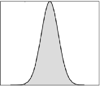
The rejection-sampling approach is illustrated in
Figure 5.10
for the example of
Illustration 1. Here, the constant
c
is chosen as [max
L
µ
ϕ
− 1
0 0022 The observation
domain is shown by the shaded area on the left side. All samples that fall into this domain
are accepted; these accepted samples follow the posterior distribution. This is verified on the
right side of
Figure 5.10
,
where the empirical CDF of the accepted samples is compared with
the analytical solution of Illustration 1.
( ]
.
.
Samples and observation domain
Posterior CDF
(a)
1
(b)
1
0.8
0.8
0.6
0.6
p
0.4
0.4
h
(μ
μ
,
p
) < 0
Empirical
0.2
0.2
Exact
0
0
15
20
25
30
35
15
20
25
30
35
μ
φ
(°)
μ
φ
(°)
Figure 5.10
Simple rejection sampling for the example of Illustration 1. (a) Samples from the prior distribu-
tion of
μ
μ
and
P
. The shaded area is the domain {(
µ
ϕ
≤
0 all samples within this domain
are accepted. (b) Empirical CDF obtained from the accepted samples, together with the exact
solution (normal CDF with mean 26.08° and standard deviation 1.39°).
hp
,)
};


Search WWH ::

Custom Search