Biology Reference
In-Depth Information
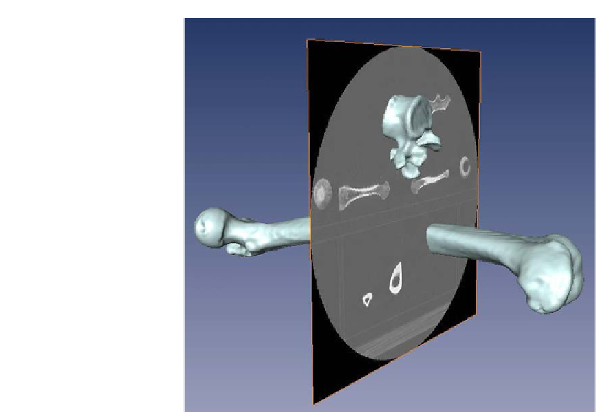
FIGURE 14.5
Segmentation
of a femur
in Amira
with
a segmented femur model.
values of gray (which are measured in Hounsfield units after the inventor, as mentioned
previously) as a criterion. This shades in the selected area of interest, similar to the “fill”
command in most photo editing programs. The voxel grayscale values therefore correspond
to the different densities of the object scanned. See
Figure 14.5
.
In Amira
, the entire shaded area can then be selected and enclosed in a colored outline.
This area of interest is termed a “label.” Because bone densities between the diaphysis and
the epiphyses are very different in densities and thus have different gray values, it may leave
open holes in the surface of the model if the threshold is set too narrowly. If the threshold is
set too broadly, it may interpret any adhering soft tissues as part of the bone, for example. The
researcher can therefore manually segment each epiphysis. Once both proximal and distal
slices are given the same label, a simple click on the same gray value anywhere in between
will automatically detect the rest of the cortical bone. It is necessary to check through each
DICOM slice of your new model to verify that the entire bone was accurately selected. Auto-
matic segmentation follows a similar format. The main distinction is that the maximum and
minimum thresholds for every slice are set simultaneously. This saves a great deal of time,
but renders poorer models, due to the vastly different densities in compact and trabecular
bone. This process of segmentation will likely become more sophisticated and completely
automatic in CT scans in the near future. For now, it is a crucial step in the process of creating
computer bone models.