Biology Reference
In-Depth Information
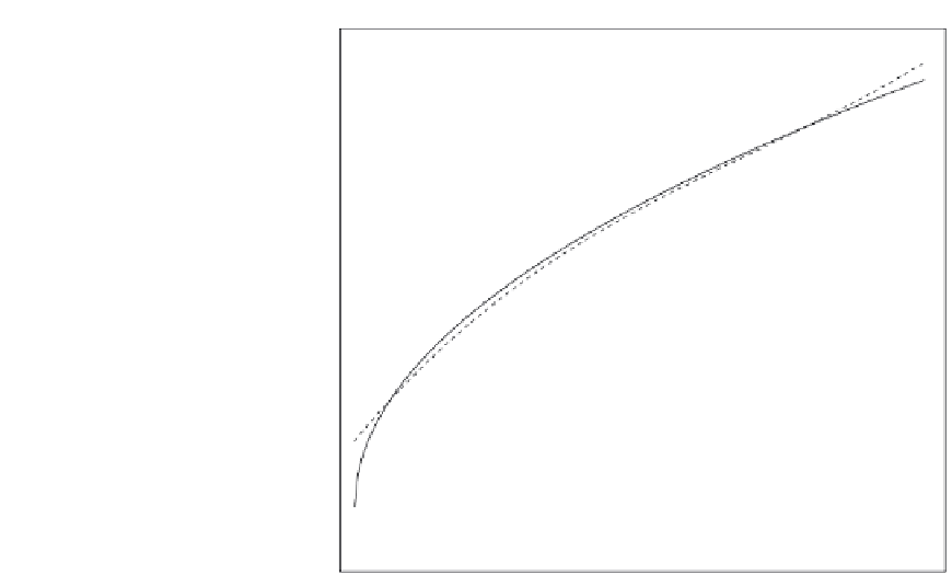
FIGURE 11.6
Plot of
mean femoral length against
age in boys. The filled points
are from
Maresh's (1970)
radiographic study, the
dashed line was fit as a third-
degree polynomial, and the
solid line was fit using frac-
tional polynomials.
0
2
4
6
8
10
12
Age
standard deviation
¼ 0:52 þ 0:11
age.
Figure 11.7
shows a plot of the mean femur length
plus and minus two standard deviations as a continuous curve from birth to age 12 years. To
simulate long bone lengths based on the hazard model age-at-death structure, we simulate
250 deaths from the exponential hazard model with the hazard parameter equal to 0.34.
We then take the simulated age-at-death for each “individual” in this dataset and simulate
a femur length using a draw from a normal distribution with the mean and standard devi-
ation predicted for the given age.
Estimating the Age-at-Death Structure
To estimate the age-at-death structure of an actual skeletal sample we write the log-likeli-
hood for obtaining the observed (or in our case, simulated) femur length data conditional on
the exponential hazard parameter. For an individual femur length (FL) measurement
the point probability of getting that measurement conditional on the exponential hazard
parameter is
Z
f
ðFLjlÞ¼
fðFLjageÞ l expðlageÞ;
(11.17)
t
where the integration is across age, for which we use a lower limit of exp(
e
10), which is
approximately 4.5
10
5
years and an upper limit of exp(3.4) or approximately 30 years.