Biology Reference
In-Depth Information
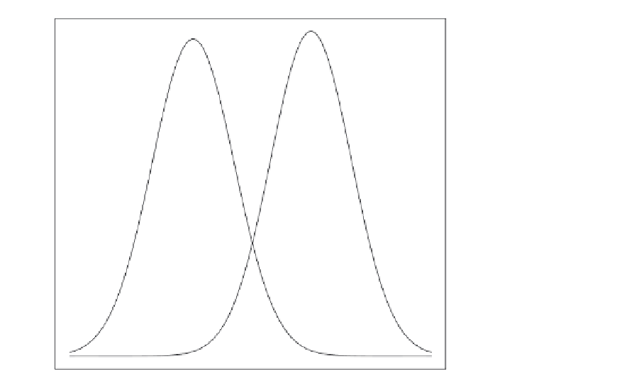
FIGURE 11.1
Normal
densities for male and for
female femoral circumfer-
ences (in millimeters). The
summary statistics for
drawing these two densities
are from
Black (1978)
, and the
vertical line is the “sectioning
point” (at 57 mm) that could
be used to sex individuals as
male versus female.
M
F
40
50
60
70
Femoral Circumference (mm)
0:9 fðx; 51; 4:2Þ0:1 fðx; 63; 4:1Þ¼0;
(11.9)
for the sectioning point x, in which case we find that the correct sectioning point should be
60.2, which we round down to 60 mm.
Figure 11.2
shows a plot of this new situation. In Equa-
tion
11.9
the
symbol is the normal density evaluated at point “x” with the specific mean and
standard deviation. Using this new sectioning point, we find that 882 females have values
less than 60 mm, 8 have a value of 60 mm, and 10 are above 60 mm. For males, 17 have values
below 60 mm, 6 have a value of 60 mm, and 77 are above 60 mm. This gives our estimated
proportion of males as (4
þ
10
þ
3
þ
77)/1000
¼
0.094, close to the correct value of 0.1. So we
needed to have some form of information about the sex ratio
f
we ever began trying
to sex individual femora. When we assumed a 50:50 sex ratio we got biased results in the
application to a sample where the real ratio was 10:90.
Since we do not always have access to the correct proportion of males when conducting
demographic analysis of actual skeletal data, MLE is a useful approach. The log-likelihood is
before
ln LK ¼
N
i ¼1
logðp
m
ffx
i
; 63; 4:1gþð1 p
m
Þffx
i
; 51; 4:2gÞ:
(11.10)
Here, the proportion of males and proportion of females are each multiplied by
a normal density based on the observed mean and standard deviation, instead of by
a matrix of trait score probabilities as in the ordinal categorical case. Using “maxLik”