Database Reference
In-Depth Information
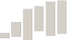
Performance gain in the BMS−2 dataset
Performance gain in BMS−1 dataset
250
400
T
SIA
T
solve
T
serial
T
SIA
T
solve
T
serial
350
200
300
250
150
200
100
150
100
50
50
0
0
2x2
2x3
2x4
3x2
3x3
3x4
2x2
2x3
2x4
3x2
3x3
3x4
Hiding Scenarios
Hiding Scenarios
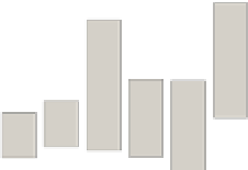
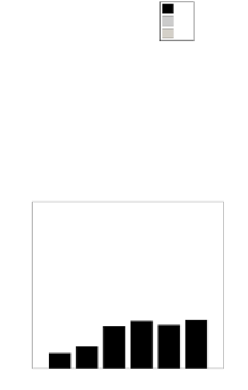
Performance gain in the Mushroom dataset
T
SIA
T
solve
T
serial
100
90
80
70
60
50
40
30
20
10
0
2x2
2x3
2x3
3x2
3x3
3x4
Hiding Scenarios
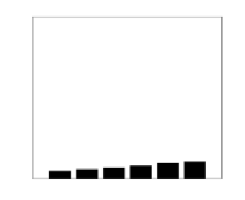
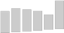
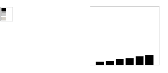
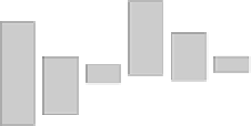
Fig. 17.7: Performance gain through parallel solving, when omitting the V part of
the CSP.
lution calculation overhead (T
aggregate
) are considered to be negligible when com-
pared to these runtimes. Moreover, the runtime of (i) does not change in the case of
parallelization and therefore its measurement in these experiments is of no impor-
tance. To compute the benefit of parallelization, we include in the results the runtime
T
serial
of solving the entire CSP without prior decomposition.
The first set of experiments (presented in
Figure 17.7)
breaks the initial CSP
into a controllable number of components by excluding all the constraints involving
itemsets from set V (see Figure 14.2). Thus, to break the original CSP into P parts,
one needs to identify P mutually exclusive (in the universe of items) itemsets to
hide. However, based on the number of supporting transactions for each of these
itemsets in D
O
, the size of each produced component may vary significantly. As
one can observe in
Figure 17.7,
the time that was needed for the execution of the
SIA algorithm and the identification of the independent components is low when
compared to the time needed for solving the largest of the resulting CPSs. Moreover,
by comparing the time needed for the serial and the one needed for the parallel
solving of the CSP, one can notice how beneficial is the decomposition strategy in
reducing the runtime that is required by the hiding algorithm. For example, in the
22 hiding scenario for BMS-1, serial solving of the CSP requires 218 seconds,